EFDC+ Explorer · Version 13 · Beta
What’s new in EEMS 13
EEMS 13 combines several model input files into one JSON file and draws every view with a new rendering engine. It adds cut-line MPI decomposition, Custom Tracers with taste and odor generation, and new analysis tools, plus improvements across hydrodynamics, water quality, sediment, boundary conditions and Grid+.
Project files
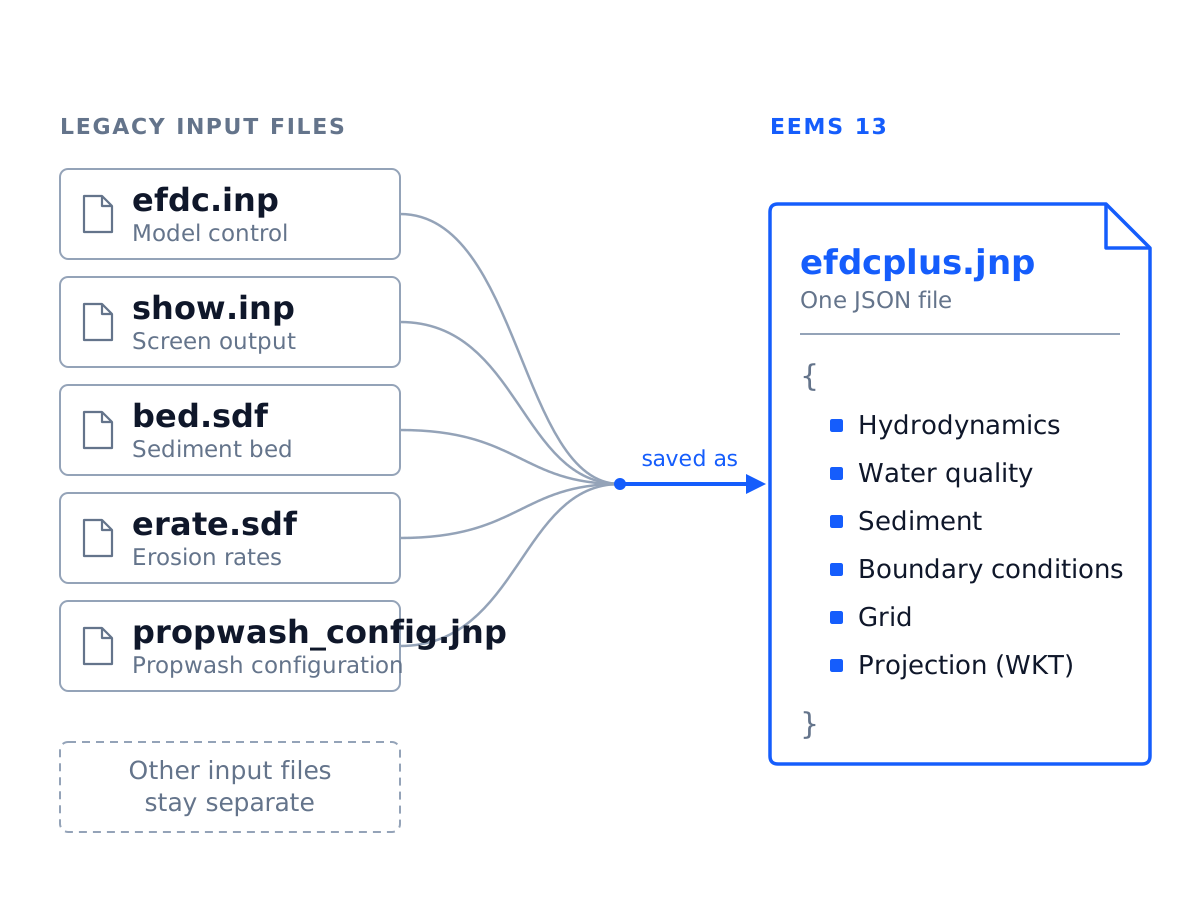
Several input files combined into one JSON file
The main control file, efdc.inp, and several module input files are now combined into a single efdcplus.jnp file. The model’s other input files stay separate.
- Version 13 no longer uses
efdc.inp, but models from earlier versions, which all use it, still open and convert automatically - The full projection is stored with the model, including WKT for user-defined projections
- New Project starts clean instead of copying files from the current folder
- Restart files are copied with the model rather than regenerated
MPI domain decomposition
MPI Graph Topology
Rectangular blocks rarely fit a branching river or an estuary full of islands, so some sub-domains get far more cells than others. EEMS 13 reads the grid as a connected network of wet cells and lets you split it along the channel.
- Draw cut lines on the Cell Map, with ends that snap to the banks
- Drag a segment and watch the cell counts on both sides update
- Balance places the cuts for you, evening out work per rank and keeping the boundary between ranks short
- Islands, tributaries and cell connectors are handled automatically
- Merge, detach or split sub-domains from the right-click menu
- Saved to
decomp.jnpand launched from the Run dialog. The block method is still available, now balanced by work.
Drag a cut segment and the cell counts on both sides update as it moves.
Right-click a sub-domain and choose Merge into to join it to another one.
Custom Tracers · Taste & Odor
Track taste and odor compounds from bloom to intake
Dye is now Custom Tracers, with as many classes as a study needs. Algal and zooplankton groups can release compounds such as geosmin as daughter products, each carried by a tracer you can map and plot.
- Tracer types: conservative, non-conservative with zero- and first-order decay, age of water, and benthic
- Dissolved or particulate phase, settling, volatilization and burial for each class
- Linked benthic and water-column classes, in units such as ng/L and g/m²
- Turn on Daughter Product Generation for any algal or zooplankton group and link a tracer
- Set stoichiometry, particulate fraction and metabolism factor for each compound
- Map the compound in 2DH and plot it over time at an intake
Dissolved geosmin moving through a reservoir over three and a half days, with the river inflow and the water intake marked.
Visualization
A new rendering engine behind every map
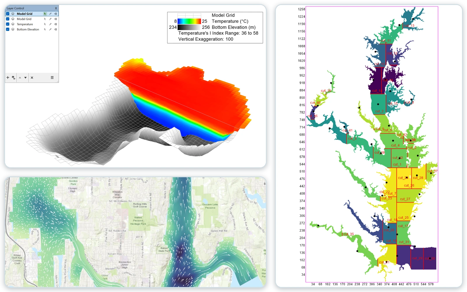
2DH, 3D, the Cell Map and Grid+ now draw with one OpenGL/Skia engine, and legends and colour bars stay sharp at any resolution.
- A new Layer Manager panel for 2DH, 3D and the Cell Map, with visibility and label toggles on each layer
- 3D smooth-field volumes build 4–6× faster
- An orbit camera that keeps the model framed when you change vertical exaggeration
- Transparency, face culling and the sediment bed in 3D volumes
- High-DPI scaling across the application
The orbit camera circles a 3D temperature volume over a reservoir's bottom elevation at 100× vertical exaggeration.
2D views
Streamlets and clearer 2D maps
Animated streamlets show the flow on 2DH maps, and 2DV gets smooth contouring that respects thin barriers.
- Streamlets: animated arrows along velocity vectors, coloured by any field, with adjustable density and fade
- A boundary-condition flux layer in 2DH, with control for each group
- Drag point scatter, label files, Grid+ files and maps straight onto a 2DH map
- Horizontal or vertical legends, with display units set for each parameter
- Animate to file, pause and stop, with output dates in the title
- Multi-point path measurement in 2DH and Grid+
Streamlets follow the tidal flow over a 2DH bottom-elevation map, with the streamlet entry shown in the legend.
Analysis
New ways to check and compare runs
Follow how a model’s wet area and volume change through a run, check its mass balance, and compare several models in one plot.
- Model Statistics: wet area, wet cell count, volume and average depth over time, with CSV export
- Mass balance from
EE_BC.OUT, with progress and a Stop button - Time series from several models in one plot, with a base-model picker
- Faster charts that break lines at data gaps and snap axis ticks to round values
- Calibration stations entered by I/J, with a time tolerance and date offset for vertical profiles
- Reports for initial conditions by layer and class, boundary series and harmonics
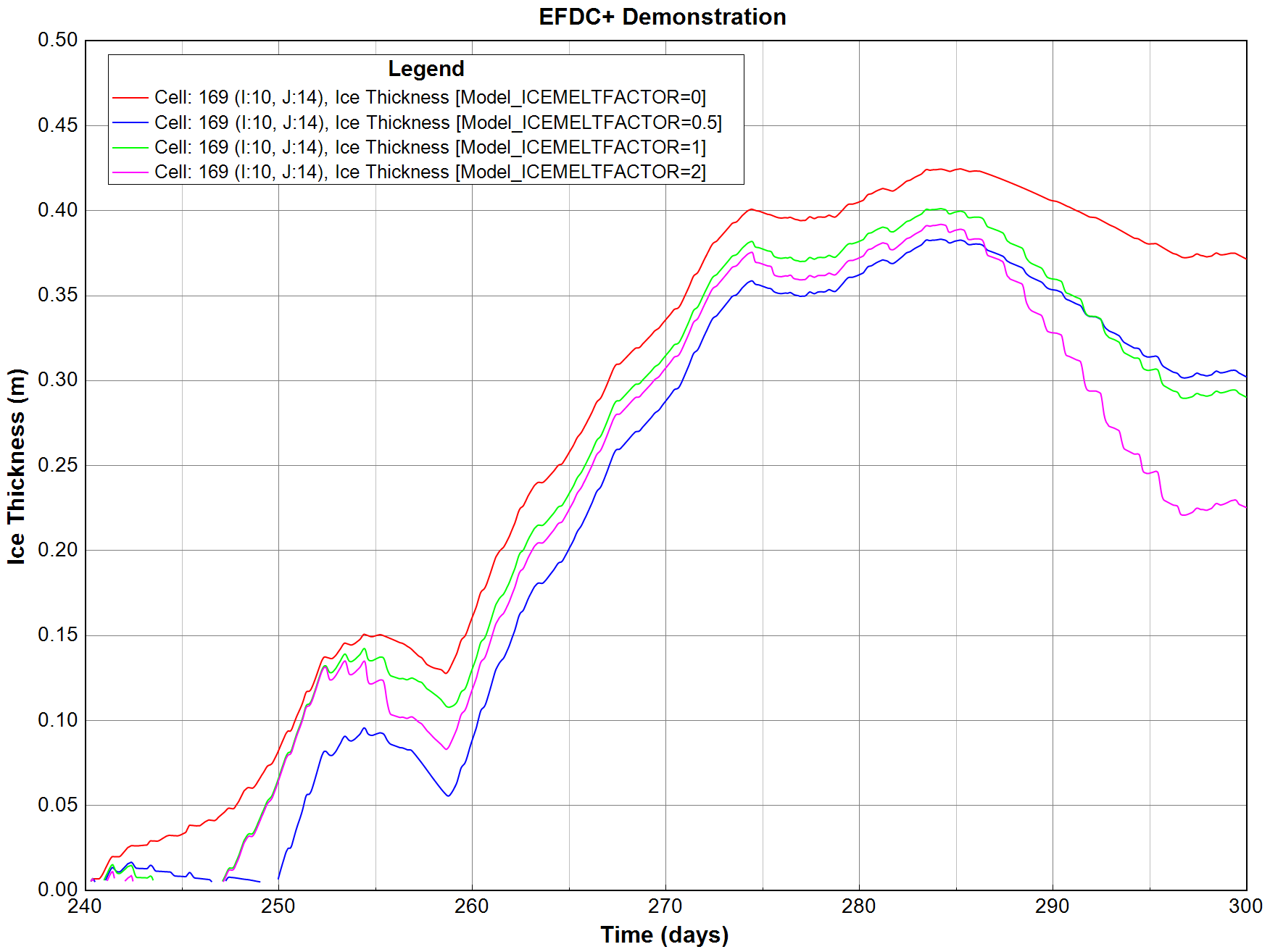
Ice thickness at one cell from four runs, each with a different ice melt factor, compared in one time-series plot.
Across the release
More changes worth knowing
Version 13 also reworks most of the model setup forms. These are the changes most users will notice.
Hydrodynamics
- Dynamic time stepping for 2TL and 3TL, with a minimum step, ramp-up and maximum growth factor
- Spatially varying Coriolis with graphical assignment and viewing
- Clear treatment of wall drag, with free-slip, partial-slip and no-slip wall conditions
- Evaporative losses, solar shading, COARE heat exchange and groundwater
- Hydraulic structures in groups, with rating lookup tables and flow split
Water quality and ChemFate
- ChemFate replaces Toxics, with atmospheric deposition, organic-carbon options and per-class bed and water initial conditions
- Added “macrophyte or benthic algae” and actinobacteria biota groups; actinobacteria grow on carbon and oxygen alone, without taking up nitrogen or phosphorus
- N2 fixation for biota groups, and zooplankton settling and ingestion rates
Sediment
- Rebuilt cohesive, non-cohesive, SEDZLJ, SedORG and fluid mud modules
- New sediment-water initial conditions and a spatial POC fraction
- SEDZLJ maximum bed layer thickness, with effective diameter in microns
- Reworked settling and diagenesis forms
Boundary conditions
- “Flow” boundaries are now called “Point Source”
- Point sources can pair a constant or time-series flow with constant or time-series concentrations, in any combination
- Mass loading at point sources for any constituent, not just water quality
- Open-boundary harmonics set per series, with face numbering that matches EFDC+
- Withdrawal/Return with pump rules, controlling series and discharge modifiers
- Duplicate BC groups, filter by BC type, and a Combine Series dialog
Grid+ and coordinates
- Grid refinement factors can be decimals, such as 1.5, not just whole numbers, for finer control of grid spacing
- Export an EFDC+ 13 model, or update an existing model’s grid in place
- Cartesian, UTM and user-defined projections, with checked conversions
- Convert cell I/J to X/Y in the Conversion Utility
Propwash and AIS
- Fill missing vessel fields by vessel group from an AIS vessel-type table
- Update ships online, including tug propeller details
- Propwash reporting, and lat/long tracks converted to UTM automatically
- Warnings for duplicate MMSI numbers
Running models
- More pre-run checks, covering waves, wetting and drying, and ice
- A warning when the control file and series files disagree
- A Restart Flags form, and restarts that work when modules are turned off
- Core count set automatically, and a Run ID tied to the run folder
- Run logging that automatically tracks changes to the input files between runs and saves
Interface
- A new icon set that stays crisp at any display scaling
- Searchable work logs, with error and warning filters
- Versioned F1 help that opens in your browser
- Accessibility support on custom controls and high-visibility scrollbars
Get EEMS 13
Download the beta installer, or read every change in the full release notes.