Closing the water budget is a crucial first step in hydrodynamic modeling of closed systems such as lakes and reservoirs. Part of the budget, however, is almost always missing from the model inputs. Ungauged contributions, such as runoff from the near-shore area and small tributaries, groundwater seepage into or out of the water body, and unmetered withdrawals, are rarely measured. Gauged flows carry their own errors, for example from rating curves extrapolated beyond the measured range or from gauges sited upstream of the lake that miss part of the drainage area, and evaporation is usually estimated rather than measured. Because the water level integrates these errors over time, even a small persistent imbalance grows into a large drift. Without a closed water balance, subsequent simulations, from water quality to sediment transport, produce unreliable results that cannot support effective management of these water bodies.
A common workaround is to scale gauged inflows by trial and error until the modeled water level looks right, which distorts the measured data and still misses the timing of ungauged contributions. This practice can be replaced by EEMS’s Reservoir Water Balance Tool. Using the model’s inflows, outflows, precipitation and evaporation, with an observed water level record as the control, the tool computes a single balance flow that accounts for all unmeasured gains and losses. The water budget is closed in one step, the gauged flows remain untouched, and the unexplained water is isolated in one series that can be inspected.
How it works
Lumping all residual flows into a single balance flow B, the water budget is:
where I is inflow from tributaries and other point sources, P is precipitation on the water surface, B is the net balance flow, E is evaporation, O is outflow through the outlet and any withdrawals, and ΔS is the change in stored volume. All terms are volumes over the balance interval, with B positive when water enters the water body.
In practice, tributary gauges, outlet records and meteorological data provide I, O, P and E, and a stage gauge provides ΔS once the water level change is converted to a volume. Everything left unmeasured, including ungauged runoff, groundwater exchange, unmetered withdrawals and measurement error, falls into B, which can therefore be recovered as the residual:
The Reservoir Water Balance Tool applies this approach. It reads the flow boundaries defined in the EFDC+ model, integrates precipitation and evaporation from the model’s atmospheric input, and computes ΔS = AΔz from the observed water level change Δz and the control region’s surface area A. Repeating this over consecutive intervals yields a balance flow time series, which the tool writes back into the model as a flow boundary condition.
Using the tool
The tool is available under Tools in the toolbar (Figure 1) and opens the Water Balance window (Figure 2). Its options, from top to bottom, are:
Timing Options
- Time Begin / Time End — the balance period in model days from the base date; defaults to the model run period.
- Interval (min.) — the length of each balance window, i.e., the time step of the output series. Shorter intervals amplify water level noise, so the default is recommended.
- Tolerance (min.) — the half-width of the ramp joining consecutive steps, which keeps the output series single-valued in time.
Control Flow File — reserved for an external flow series not tied to a model boundary; not active in this release.
Rainfall and Evaporation — fixed to the P and E in ASER.INP.
List of Control Regions — the regions over which the budget is closed. Whole Model is created automatically from the grid area and all point-source boundary groups. Add New creates another region, and Load and Save store the configuration as JSON. Keeping the default Whole Model region is recommended.
Current Control Region
- Name — region label.
- Area (m²) — the constant surface area used to compute ΔS = AΔz and to convert precipitation and evaporation depths to volumes.
- Update Series — the flow series that receives the computed balance flow. A synthetic, readily configured balance flow is recommended.
- Number of Flow Boundaries — the number of point-source boundary groups within the region.
- Bounding Polygon — an overlay file defining a sub-region; boundary groups with cells inside it are assigned to the region. Leave empty for the whole model.
- Control Water Level — the observed water level record, the only data supplied directly to the tool. Required.
- Interval for Water Level Averaging (min.) — the window over which the water level is averaged at each interval endpoint, to suppress gauge noise and seiching.
- Control Flow — reserved; see Control Flow File.
Compute — runs the balance, updates the selected series in memory, and opens a summary report listing each series’ loading factor and integrated volume. Save the model to keep the result.
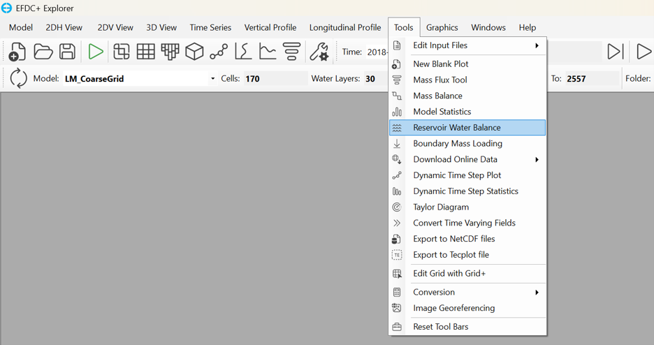
Figure 1. Opening the Reservoir Water Balance tool
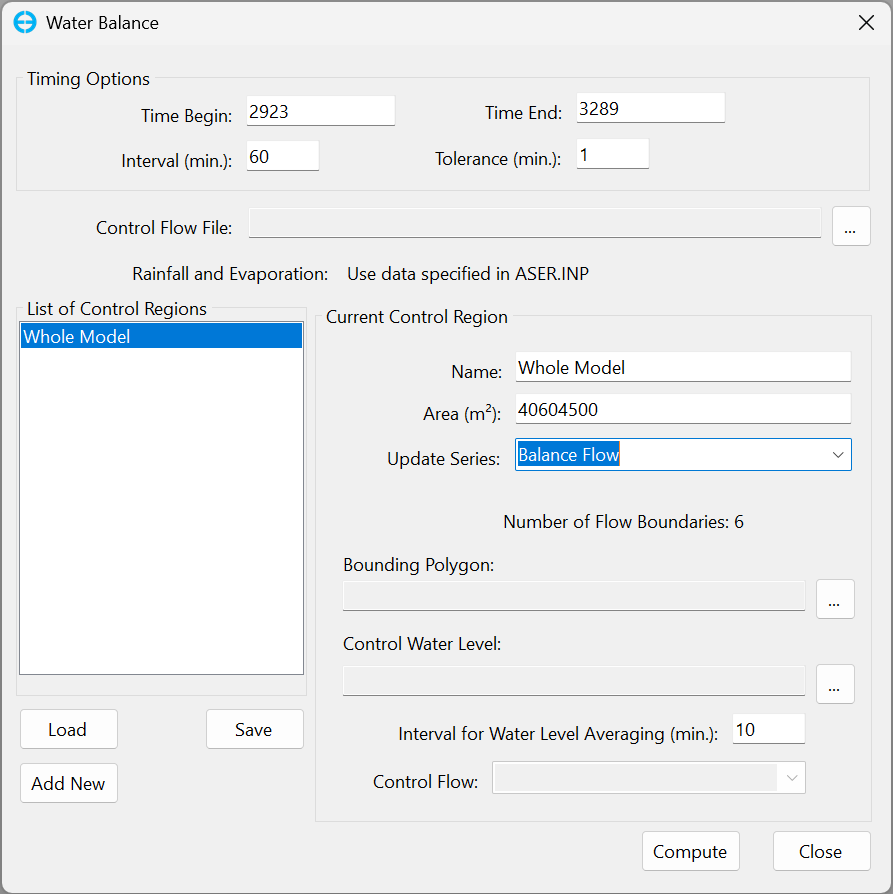
Figure 2. The Water Balance tool window
Example: Lake Mendota
Here the tool is applied to the Lake Mendota model, which had been introduced in a previous blog. The model has 1045 horizontal cells, 30 vertical layers and five point-source flow boundaries: four inflows (Yahara River, Sixmile Creek, Dorn Creek and Pheasant Branch) and one outflow. A sixth point-source boundary, Balance Flow, is assigned to a single cell to carry the computed flow. Figure 3 shows the model grid. In the setup (Figure 4), Balance Flow is selected as the Update Series, and the water level recorded at the lake outlet between 2014 and 2023 is used as the Control Water Level, with the balance computed over the 2020 simulation period.
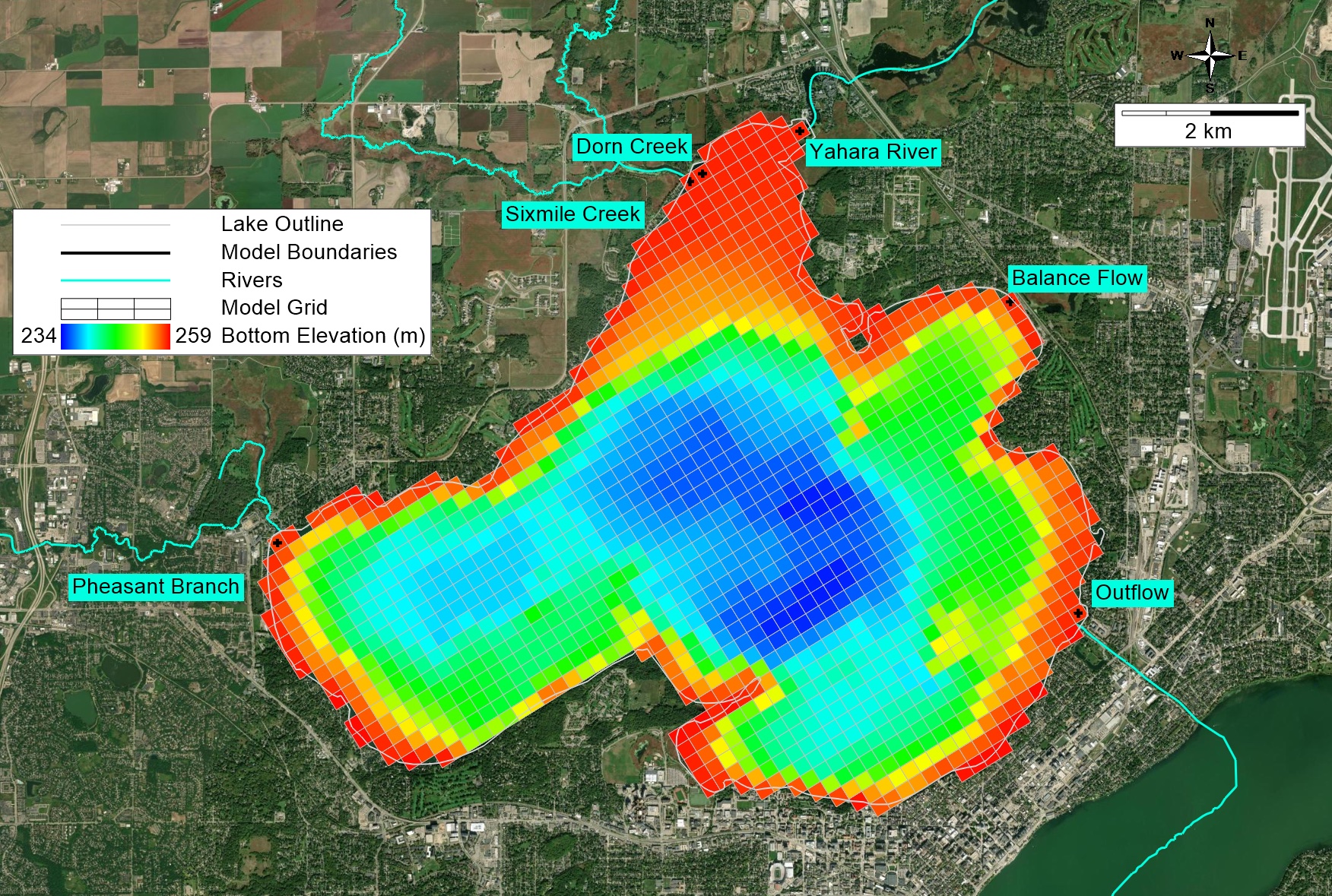
Figure 3. Lake Mendota model grid
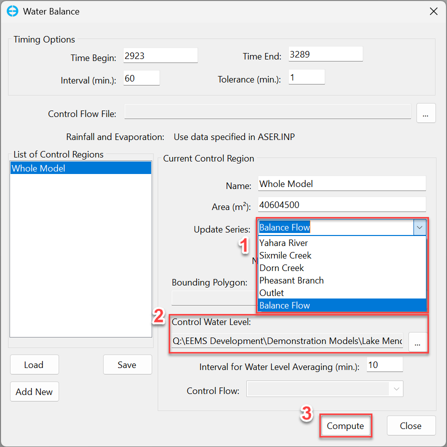
Figure 4. Computing the balance flow
Figure 5 shows the computed hourly balance flow, which averages 2.638 m³/s. The hourly values swing widely because small water level fluctuations translate directly into flow (a 1 mm change in one hour over the lake’s 40.6 km² equals about 11 m³/s); the net volume over time is the meaningful quantity. Because the balance flow is a residual, a value far larger than the expected ungauged contribution signals missing or erroneous data rather than a real flow, and points to the need for more data collection.
Figure 6 compares modeled and observed water levels at the outlet for runs with and without the balance flow. Without it, the modeled level falls more than 1 m below the observations by July; with it, the model closely tracks the observed water level, confirming that the water budget is closed.
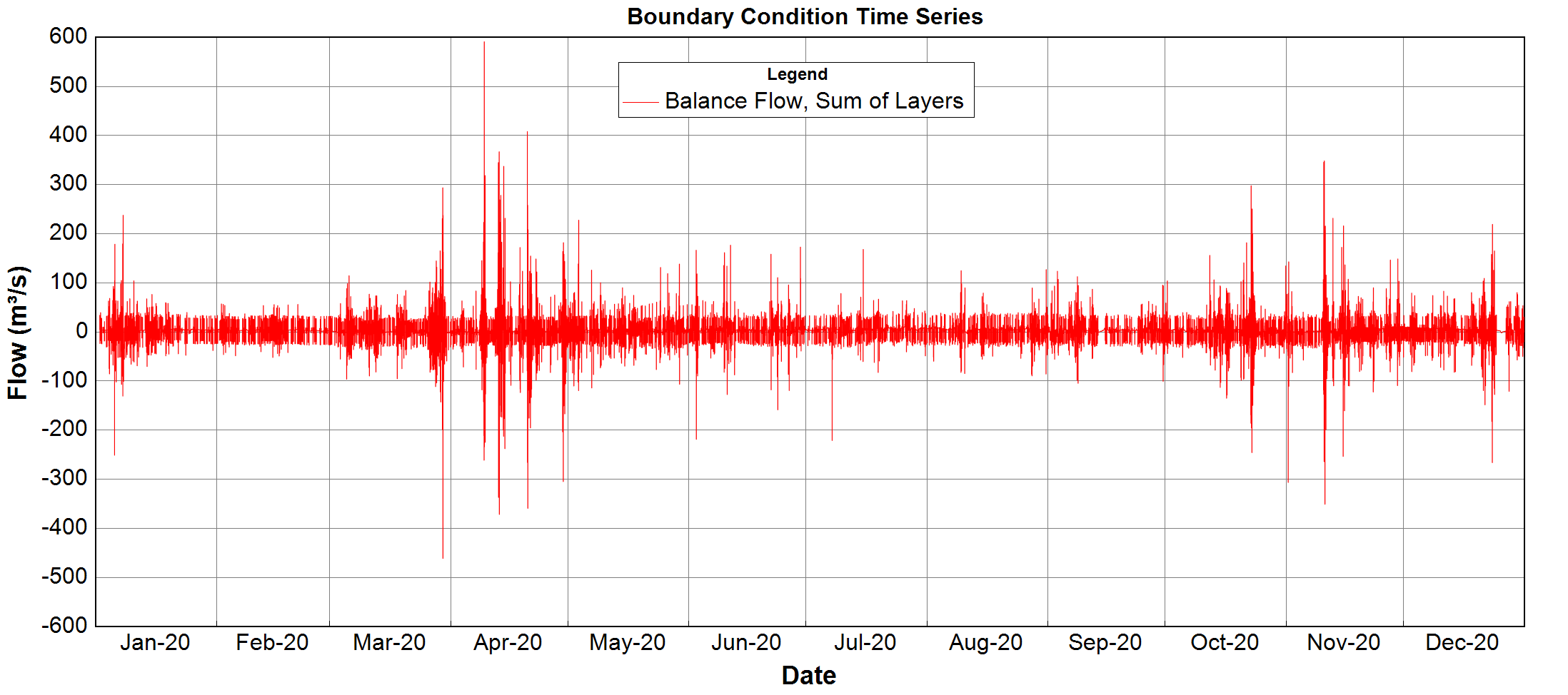
Figure 5. Calculated Balance Flow
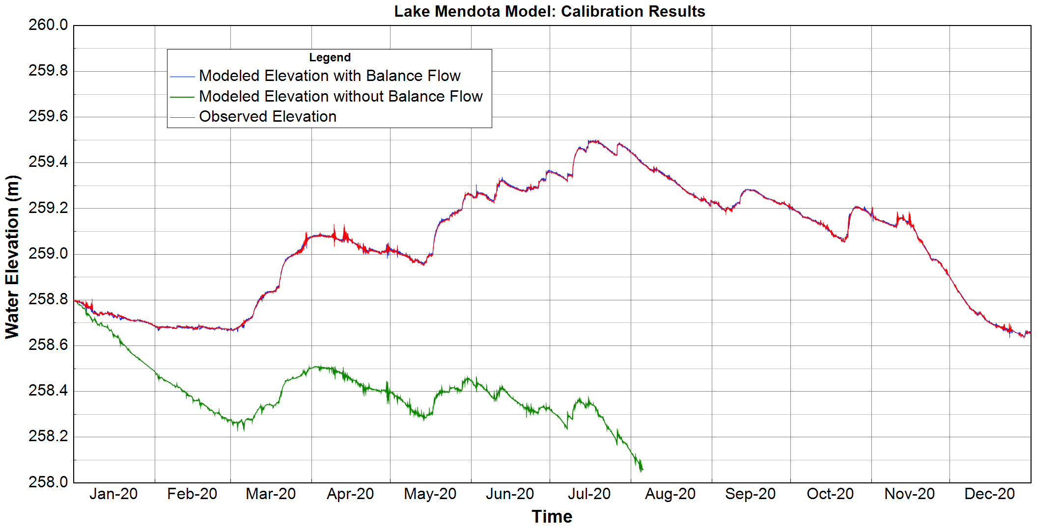
Figure 6. Time series of model outputs between model using balance flow and model without a balance flow
Limitations
The tool has two limitations. First, it applies only to models without an open boundary, where the water level is governed by point-source flows and atmospheric exchange alone. Second, the tool computes the storage change as ΔS = AΔz with a constant surface area, so for reservoirs where the surface area varies appreciably over the drawdown range, the resulting balance flow will carry a systematic error. Because the same area converts precipitation and evaporation depths to volumes, models with extensive wetting and drying are affected in the same way.
Conclusion
The Reservoir Water Balance Tool in EEMS turns a tedious, iterative calibration step into a few clicks. Given an observed water level record, it computes the balance flow that closes the water budget and writes it directly into the model, giving water quality and sediment transport simulations a sound hydrodynamic foundation. As a residual, the balance flow also serves as a diagnostic: its magnitude shows how much water the gauged data fail to explain and where further data collection is most needed.